
A transcript begins with the signal that reaches the recognizer. Before a model makes its first prediction, the microphone, radio path, receiver and capture software have already determined what evidence is available. Our existing recordings suggest a useful place to start a reliability study: distinguish speech that has been changed from speech that is missing.
Same words, different input path
Our saved evaluation contains 67 LibriSpeech utterances replayed through a radio capture path. Of these, 63 were labeled usable and four clipped. In this dataset, clipped means truncated audio: part of the utterance was cut off. It does not mean that the waveform hit an amplitude limit. We kept those groups separate and recomputed word error rate from the saved model outputs.
Across the 63 usable pairs, every tested configuration made more word errors on the radio recording than on the clean source. Granite rose from 3.63% to 6.29% WER; Parakeet TDT v3 from 2.32% to 7.01%; Whisper large-v3 from 2.75% to 6.09%; and Nemotron int4 from 4.45% to 12.02%. Across all seven configurations, the increase ranged from 2.66 to 7.57 percentage points.
This shows that the full replay and recording path added errors. It does not measure RF noise alone. The recording also includes the effects of the loudspeaker, microphone, room, gain, segmentation, and any other processing in the path. We would need paired signals or controlled tests to separate those causes.
When speech is missing
The four truncated captures show a different scale of failure. Their radio WER ranged from 45.07% to 62.91%, while the corresponding clean-source WER ranged from 0.47% to 3.76%. Depending on the model, 90 to 132 of the 213 reference words were counted as deletions. These are a small set of failure cases, but they make capture completeness impossible to ignore.
A missing word in a transcript does not prove that the word was absent from the audio. A recognizer can miss speech that is still audible. The next step is to line up each received recording with its original, mark the missing sections, and separate words lost during capture from words missed by the model. The paired WAVs were not available for this review, so we have not assigned those causes.
That distinction changes the engineering problem. Recognizing a distorted word and preventing the word from disappearing are different tasks. A system may guess a missing word from context, but a plausible guess is not proof that the audio contained it.
Reading a mel spectrogram
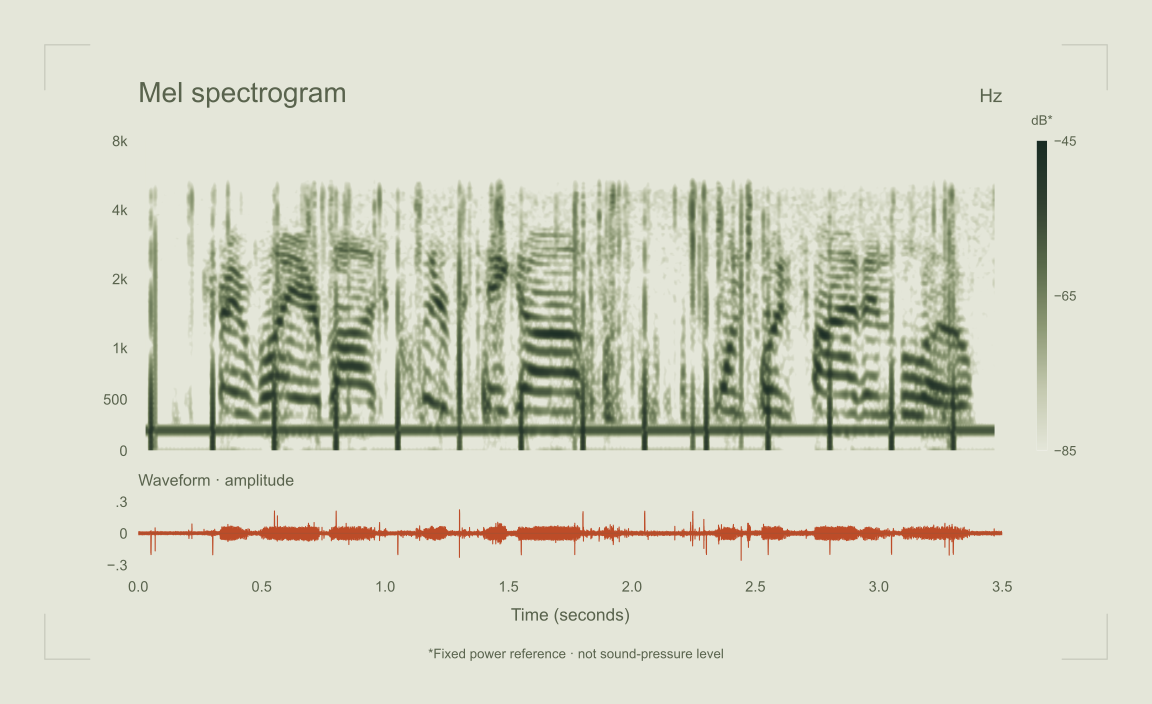
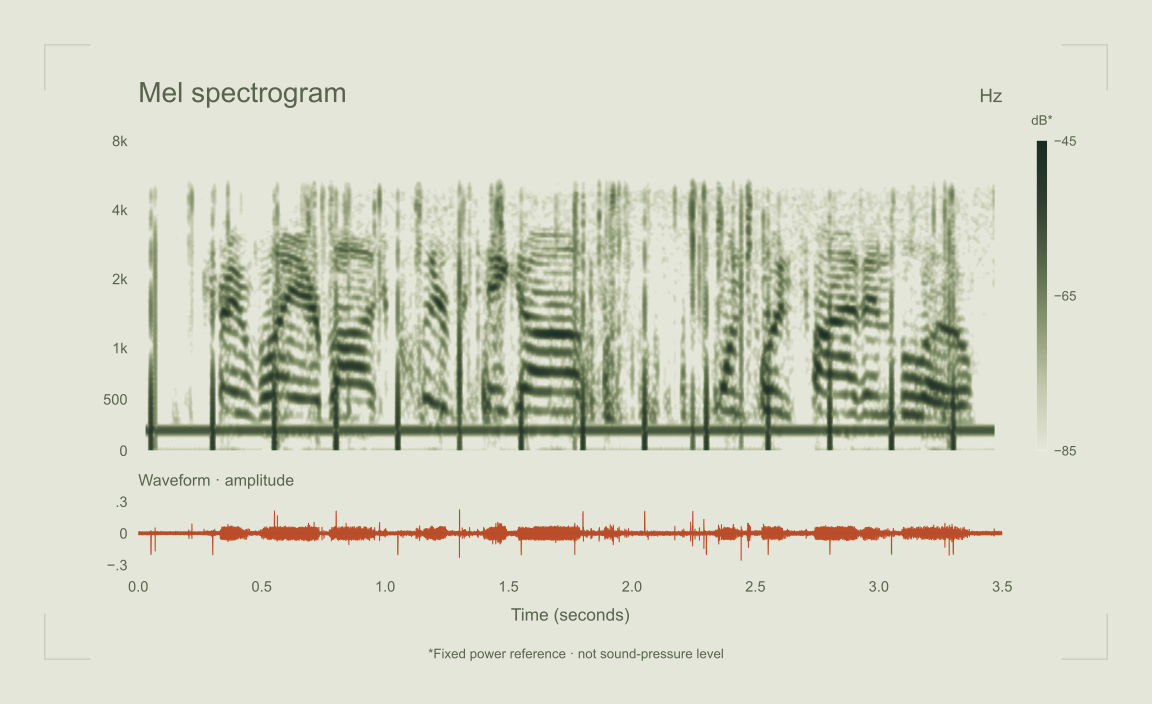
A waveform shows amplitude over time. A spectrogram breaks the signal into short overlapping windows and shows how energy is distributed across frequency. A mel spectrogram collects that energy into mel-spaced bands, allocating finer frequency resolution toward the lower part of the spectrum. The result makes patterns in speech easier to inspect, while sacrificing some fine frequency detail.[2]
In Figure 01, the mel view makes the changing harmonic structures and the persistent low-frequency component visible. The waveform makes the changing amplitude and repeated narrow transients easier to locate. A linear-frequency spectrogram would provide a complementary view of narrow tones and spectral boundaries. None of these views, by itself, identifies the speaker, supplies the missing words, or establishes why a transient occurred.
The figure uses real field audio, but it is not a clean-versus-radio pair. It also is not the exact frontend representation of every model in the evaluation. All display parameters are recorded so a later paired figure can use consistent windows, frequency limits and color scales. Normalizing each image to its own brightest point would conceal some differences in level.[2]
Noise, distortion and loss
Noise can mask speech that is still present. Amplitude saturation reshapes the waveform. Truncation removes its beginning or ending. Internal gaps interrupt it. These conditions can coexist, but collapsing them into a single label such as bad audio makes a useful diagnosis harder. NIST’s radio-audio research similarly examines the interaction between background noise and communication-system components using intelligibility measurements.[1]
Our field inventory contains 185 WAVs, totaling 312 seconds. Only 13 have automated transcript entries, and those entries are not human ground truth. Most files were automatically classified as narrow unmodulated candidates. These detector labels are not validated speech labels, so the collection should not be described as 185 verified speech examples.
None of those WAVs reached an absolute normalized sample amplitude of 0.99. That is a reproducible full-scale check, not proof that the chain never clipped: upstream saturation followed by attenuation could remain below that threshold. Similarly, a darker spectrogram after denoising does not establish better recognition. Speech-enhancement research documents the tradeoff between noise reduction, speech distortion and ASR performance.[3]
Measure what arrives, then what is understood
A channel study should retain the original audio, the received audio and their timing relationship. It should report whether the full utterance was captured before measuring how accurately it was transcribed. Missing, split, merged and truncated captures must stay visible rather than disappearing from a clean headline score.
Latency belongs in that record, but its boundaries must be explicit. Access to the channel, transport of audio, closure of a captured segment and delivery of a final transcript are separate intervals. NIST’s work on start-of-word correction shows how audio before a keyword can bias an access-time measurement. Our saved batch timings do not establish those channel intervals, so this analysis makes no channel-dependent latency claim.[4]
The next step is to recover the paired replay waveforms and annotate the four truncated cases alongside representative usable captures. That would let us connect a visible signal change to a specific word error. The contribution of this pilot is narrower: it shows why recognition reliability has to account for the evidence the capture path preserves.
Evidence boundary
Limits & open questions
- The 67-clip evaluation uses read English replayed through a radio path. It does not establish accuracy on spontaneous workplace communication.
- Only four captures were labeled as truncated. Their results are diagnostic examples, not a stable failure rate or basis for ranking models.
- The paired replay WAVs were unavailable at the location recorded in the evaluation repository during this review. We reproduced transcript scores but could not independently verify the truncation labels against those waveforms.
- The field recording shown in Figure 01 has no verified human transcript. Its visible features cannot be linked to a specific recognition error.
- The replay path combines acoustic, radio, receiver and capture effects. This analysis does not isolate an RF cause, demonstrate a latency effect, or establish how much error fine-tuning could recover.
How this article was researched
We re-scored saved clean and radio-replayed hypotheses from seven model configurations using the evaluation repository’s original normalization and alignment code. All seven headline clean/radio scores reproduced the saved board. We separately profiled 185 recorded 16 kHz WAVs and rendered the figure directly from one recording, without denoising or amplitude normalization. The mel view uses a 32 ms Hann window, 5 ms hop, 1024-point FFT and 128 bands from 0–8 kHz. Power is normalized by the squared window sum and displayed against a fixed numerical reference; the scale is not calibrated sound pressure. The excerpt was selected visually for distinct harmonic structures among the 12 field recordings at least three seconds long. The displayed power range is fixed at −85 to −45 dB; time starts at the excerpt boundary. This is an illustrative selection, not a representative sample.
Article type: measured research. This study reports a reanalysis of existing model outputs and descriptive measurements of existing recordings. No new model inference or radio transmission was performed. The field figure is measured audio, not a schematic.
Sources & further reading
Sources reviewed on 24 September 2026. “n.d.” indicates no fixed publication date for the linked version.
- Public Safety Audio QualityNational Institute of Standards and Technology · n.d.
- Mel-spectrogram representation and filterbank parameterslibrosa documentation · n.d.
- Effect of noise suppression losses on speech distortion and ASR performanceSebastian Braun and Hannes Gamper · 2021
- Mission Critical Voice Start-of-Word Correction for Access Delay Measurement SystemNational Institute of Standards and Technology · 2021